Standard Drawing: Animation and images
Images. PU standard draw library supports drawing pictures as well as geometric shapes.

• Images. Our standard draw library supports drawing pictures as well as geometric shapes. The command StdDraw.picture(x, y, filename) plots the image in the given filename (either JPEG, GIF, or PNG format) on the canvas, centered on (x, y).
• Resources:

  https://introcs.cs.princeton.edu/java/15inout/TennisBall.png 
  https://introcs.cs.princeton.edu/java/15inout/pipebang.wav

• User interaction. Our standard draw library also includes methods so that the user can interact with the window using the mouse.
  

  double mouseX() return x-coordinate of mouse double mouseY() return y-coordinate of mouse boolean mousePressed() is the mouse currently being pressed?

  • • A first example. MouseFollower.java is the HelloWorld of mouse interaction. It draws a blue ball, centered on the location of the mouse. When the user holds down the mouse button, the ball changes color from blue to cyan. A simple attractor. OneSimpleAttractor.java simulates the motion of a blue ball that is attracted to the mouse. It also accounts for a drag force.
    • Many simple attractors. SimpleAttractors.java simulates the motion of 20 blue balls that are attracted to the mouse. It also accounts for a drag force. When the user clicks, the balls disperse randomly.
    • Springs. Springs.java implements a spring system.

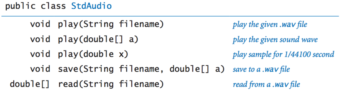
  Standard audio.

  StdAudio is a library that you can use to play and manipulate sound files. It allows you to play, manipulate and synthesize sound.

  

  We introduce some some basic concepts behind one of the oldest and most important areas of computer science and scientific computing: digital signal processing.

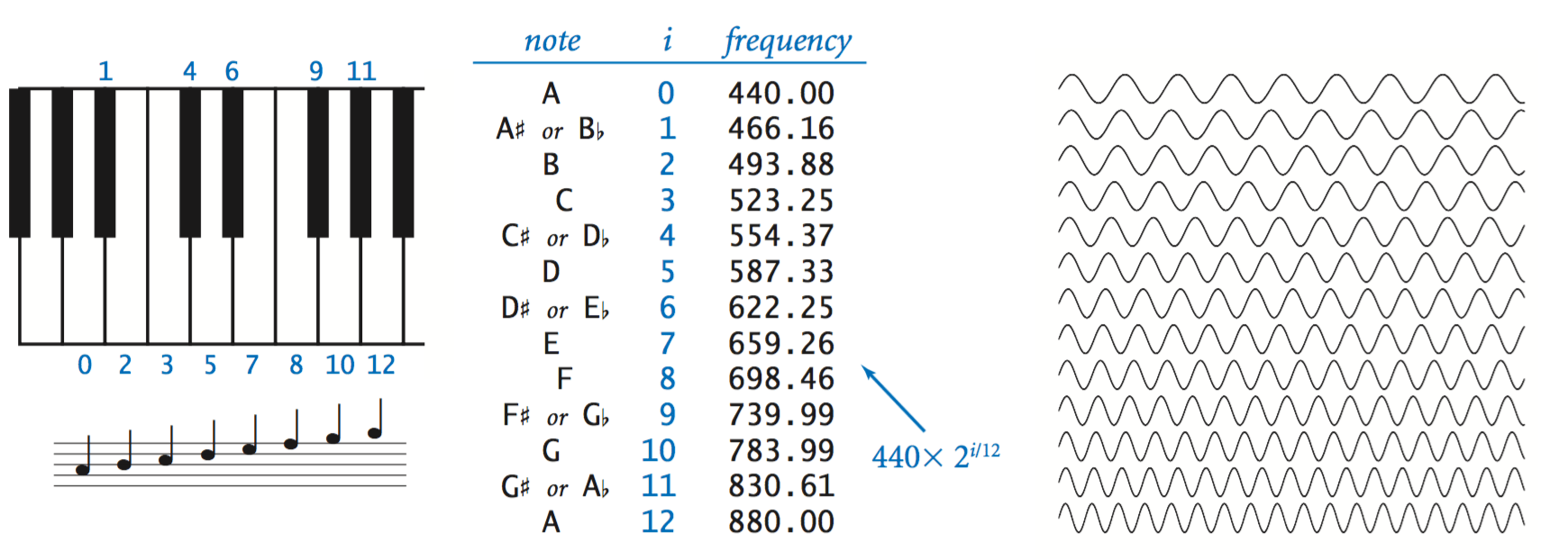
  • Concert A. Concert A is a sine wave, scaled to oscillate at a frequency of 440 times per second. The function sin(t) repeats itself once every 2π units on the x-axis, so if we measure t in seconds and plot the function sin(2πt × 440) we get a curve that oscillates 440 times per second. The amplitude (y-value) corresponds to the volume. We assume it is scaled to be between −1 and +1.
  • Other notes. A simple mathematical formula characterizes the other notes on the chromatic scale. They are divided equally on a logarithmic (base 2) scale: there are twelve notes on the chromatic scale, and we get the ith note above a given note by multiplying its frequency by the (i/12)th power of 2.

  

  • When you double or halve the frequency, you move up or down an octave on the scale. For example 880 hertz is one octave above concert A and 110 hertz is two octaves below concert A.
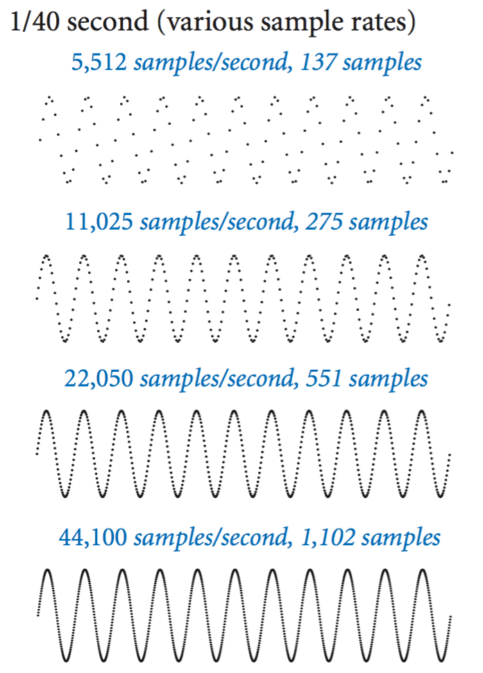
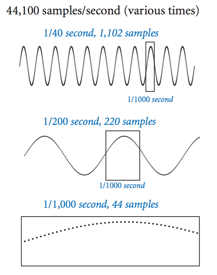
  • Sampling. For digital sound, we represent a curve by sampling it at regular intervals, in precisely the same manner as when we plot function graphs. We sample sufficiently often that we have an accurate representation of the curve—a widely used sampling rate is 44,100 samples per second. It is that simple: we represent sound as an array of numbers (real numbers that are between −1 and +1).
  •  

  For example, the following code fragment plays concert A for 10 seconds.

  int SAMPLING_RATE = 44100; double hz = 440.0; double duration = 10.0; int n = (int) (SAMPLING_RATE * duration); double[] a = new double[n+1]; for (int i = 0; i <= n; i++) { a[i] = Math.sin(2 * Math.PI * i * hz / SAMPLING_RATE); } StdAudio.play(a);

  • Play that tune. PlayThatTune.java is an example that shows how easily we can create music with StdAudio. It takes notes from standard input, indexed on the chromatic scale from concert A, and plays them on standard audio.